Practical Bayesian IRT Modeling in R

I spent a good chunk of my 5-year Political Science PhD attempting to estimate the ideology of various groups and individuals. During this time I developed a workflow for constructing the types of statistical models that purport to accomplish this, and I wanted to share some of what I have learned in this blog post. I was also recently inspired to do some ideology estimation in the context of the US Supreme Court after hearing about the debate between the 3-3-3 Court and the 6-3 Court.

This post is organized as follows:

• Section 1 provides a conceptual overview of IRT ideology models.
• If you want to skip all the Greek letters and math notation, go to Section 2 for the coding workflow in R.
• And if you only want to read the interpretation of the model results through my uninformed and half-baked analysis of the Supreme Court, skip to Section 3.

1 A Conceptual Introduction to IRT

Item-Response Theory (IRT) models are a class of statistical models used to measure latent traits in individuals.¹ These traits are characteristics which we cannot observe directly, such as height or weight, but which we instead have to infer indirectly through observed actions. For example, a student’s responses to questions on an exam might give us some idea about their latent intelligence—or a politician’s votes in Congress might give us some idea about their underlying political ideology.

Say we want to determine where a Supreme Court justice lies on a left-right ideological scale. We will call this variable \(\theta\). One place is start would be to qualitatively code each Supreme Court decision as either being liberal (0) or conservative (1), and then look at the proportion of times each justice sided with the conservative outcome. Expressed as a statistical model we get:

\[ \begin{aligned} y_{ij} \sim \text{Bernoulli}(\Phi(\theta_i)) \end{aligned} \tag{1}\]

Where whether each justice sides with a conservative decision (\(y_{ij}\)) is based probabilistically on the (scaled) proportion of conservative positions (\(\theta_i\)). The Standard Normal cumulative distribution function (\(\Phi\)) is there to add some random noise in the model. We don’t want our ideology measurements to be deterministic based on past decisions. Instead, we want to allow some room for some idiosyncratic errors to occur. On even the most conservative possible decision, we allow for some tiny probability that Clarence Thomas takes the liberal side. The Bernoulli distribution turns the probabilities produced by the \(\Phi\) function into observed 0’s and 1’s (liberal or conservative votes). See my post on Probit regression models for more on this.

The model in Equation 1 has at least one major flaw. Because there are only parameters for justices (\(\theta_i\)) and none for cases, it treats all cases before the Supreme Court as interchangeable. Additive index variables such as these implicitly assume that each “item” (i.e. case) contributes the same amount of weight towards measuring the latent construct in question. In the example of the Supreme Court this is clearly a bad assumption to make since some cases clearly have more ideological importance than others.²

Let’s fix this flaw by adding a case-level parameter (\(\xi_j\)) to the model:

\[ \begin{aligned} y_{ij} \sim \text{Bernoulli}(\Phi(\theta_i + \xi_j)) \end{aligned} \tag{2}\]

Equation 2 is commonly known as the 1-Parameter IRT Model.³ Each case now has an independent latent variable for how likely every justice is to vote in the conservative direction. For IRT models within the context of standardized tests, \(\xi\) is called the “difficulty” parameter—questions on exams vary in how difficult they are to answer correctly.

The 1-Parameter IRT model in Equation 2 is a big improvement over the additive index model in Equation 1, but if we want to be serious about measuring Supreme Court justice ideology we need to go further.

\[ \begin{aligned} y_{ij} \sim \text{Bernoulli}(\Phi(\gamma_j\theta_i + \xi_j)) \end{aligned} \tag{3}\]

The 2-Parameter IRT model in Equation 3 adds one more case-level parameter (\(\gamma\)) which allows the ideological valence of each case to vary. In the test-taking context, \(\gamma\) is referred to as the “discrimination” parameter. What this means in the context of the Supreme Court is that we expect certain cases to more strongly separate liberal justices from conservative justices.⁴

The 2-Parameter IRT model in Equation 3 was originally developed and applied to Supreme Court justices by Martin and Quinn (2002). For an excellent overview on the latest in judicial ideology measurement methods see Bonica and Sen (2021).

2 Step-by-Step IRT Modeling in brms

Now let’s turn to coding up the IRT model in Equation 3, and use it to measure the ideology of Supreme Court justices. There are three steps to this process:

1. Prepare the data
2. Build the model (and check the model)
3. Extract the ideology estimates

library(dplyr)
library(brms)
library(tidybayes)
library(ggplot2)
library(ggdist)

2.1 Prepare the data

The Washington University Law Supreme Court Database is a fantastic resource for data on Supreme Court cases. We will be using the justice centered data because ultimately it is justice characteristics we care about.

votes <- readr::read_csv(here::here("posts", "irt-brms", "data-raw", "SCDB_2023_01_justiceCentered_Vote.csv"))

The votes data frame contains justice voting data stretching back to 1946. It is already in “long format”, which is great because that’s what works best with our modeling approach using the brms R package. By long format we mean that every row contains a unique justice-case pair.⁵

votes_recent <- votes |> 
  filter(term == 2022) |> 
  mutate(direction = case_when(direction == 2 ~ 1,
                               direction == 1 ~ 2,
                               .default = NA))

Next we will filter out all years except for the 2022 term because this is where the 3-3-3 vs 6-3 debate is taking place. Lastly, we will recode the outcome variable, direction, such that 2 represents the conservative position and 1 represents the liberal position. This helps align liberal with “left-wing” and conservative with “right-wing” on the unidimensional ideology scale we are building. The method behind coding a decision as liberal versus conservative is explained in more detail here.

2.2 Build the model

With our data ready to go it is time to translate the model from Equation 3 into R code. The brms R package makes constructing the model, as well as extracting the results, relatively straightforward.⁶

irt_formula <- bf(
  direction ~ gamma * theta + xi,
  gamma ~ (1 | caseId),
  theta ~ (1 | justiceName),
  xi ~ (1 | caseId),
  nl = TRUE
)

We start with writing out the formula for our ideology model: irt_formula. The top line direction ~ gamma * theta + xi translates Equation 3 into code with the direction variable—whether a justice took a conservative or liberal position on a case—swapped in for \(y_{ij}\). Each of gamma, theta, and xi are modeled hierarchically using either the case variable caseID or justice variable justiceName. Hierarchical modeling allows each of these three parameters to partially pool information from other cases or justices, which imposes regularization on the estimates and improves out-of-sample fit. This should be the default practice whenever building an IRT model. Lastly, the line nl = TRUE is necessary because the term gamma * theta means that our model is “non-linear”.

Priors are important in all Bayesian models, but they are especially important for IRT due to these models’ inherently tricky identification problems. A model is “properly identified” if, given a specific set of data, the model will produce a unique set of plausible parameter values. As it currently stands this is not the case for either Equation 3 or its code-equivalent irt_formula. Identification is difficult for IRT models because there is no inherent center, scale, or polarity for latent variables. It might be natural to think of 0 as the center for ideology, but nothing in Equation 3 makes that so. Likewise, there is no one way of telling how stretched out or compressed the ideology scale should be. And finally, there is nothing to tell us whether increasing values should correspond to ideology becoming more liberal or to becoming more conservative (polarity).

irt_priors <- 
  prior(normal(0, 2), class = b, nlpar = gamma, lb = 0) +
  prior(normal(0, 2), class = b, nlpar = theta) +
  prior(normal(0, 2), class = b, nlpar = xi)

We will solve each of these three identification problems by setting a few priors on the parameters. Each of gamma, theta, and xi will get relatively narrow Normal(0, 2) priors. These encode a default center and scale into the model. Lastly we set lb = 0 on gamma which means that its lower-bound cannot be less than zero, and therefore gamma must be positive for all cases. This, in conjunction with defining the direction variable such that higher values = conservative and lower values = liberal, fixes the polarity identification problem.

get_prior(
  formula = irt_formula, 
  data = votes_recent, 
  family = bernoulli(link = "probit")
)

For help setting priors in brms you can use the get_prior() function with your formula, data, and model family. It will tell you what the default priors are for this model. To solve the identification problems in irt_formula we only need to set priors on the class = b intercepts, but if you wanted to get a little more fancy you could add custom priors to the class = sd scale parameters (the default Student t(3, 0, 2.5) seems fine to me).

irt_fit <- brm(
  formula = irt_formula,
  prior = irt_priors,
  data = votes_recent,
  family = bernoulli(link = "probit"),
  backend = "cmdstanr",
  cores = 8,
  threads = threading(2),
  control = list(adapt_delta = 0.99,
                 max_treedepth = 15),
  refresh = 0,
  seed = 555
)

Running MCMC with 4 chains, at most 8 in parallel, with 2 thread(s) per chain...

Chain 4 finished in 33.1 seconds.
Chain 1 finished in 34.5 seconds.
Chain 2 finished in 39.3 seconds.
Chain 3 finished in 43.8 seconds.

All 4 chains finished successfully.
Mean chain execution time: 37.7 seconds.
Total execution time: 44.0 seconds.

Let’s finally add our IRT formula, priors, and data into the brm() function and fit the IRT model. The brm() function takes these inputs and translate them in Stan code which is run using backend = "cmdstanr".⁷ The default four chains will sample in parallel if you set cores = 4 or greater. Combining cores = 8 with threads = threading(2) allows two of your cores to work on each chain, which can help speed up the sampling. The adapt_delta = 0.99 and max_treedepth = 15 options give the sampler a bit more oomph, to use a technical term. This will help make sure things don’t run off the rails due to identification issues during sampling—which can still creep up in IRT models despite our best efforts in setting priors.

summary(irt_fit)

 Family: bernoulli 
  Links: mu = probit 
Formula: direction ~ gamma * theta + xi 
         gamma ~ (1 | caseId)
         theta ~ (1 | justiceName)
         xi ~ (1 | caseId)
   Data: votes_recent (Number of observations: 623) 
  Draws: 4 chains, each with iter = 2000; warmup = 1000; thin = 1;
         total post-warmup draws = 4000

Multilevel Hyperparameters:
~caseId (Number of levels: 55) 
                    Estimate Est.Error l-95% CI u-95% CI Rhat Bulk_ESS Tail_ESS
sd(gamma_Intercept)     1.64      1.11     0.31     4.59 1.00      959     1366
sd(xi_Intercept)        2.81      0.69     1.62     4.26 1.01      355     1091

~justiceName (Number of levels: 9) 
                    Estimate Est.Error l-95% CI u-95% CI Rhat Bulk_ESS Tail_ESS
sd(theta_Intercept)     1.51      1.24     0.33     4.38 1.00     1566     2099

Regression Coefficients:
                Estimate Est.Error l-95% CI u-95% CI Rhat Bulk_ESS Tail_ESS
gamma_Intercept     1.07      0.72     0.20     2.91 1.00     1417     1569
theta_Intercept    -1.02      1.10    -3.39     1.15 1.02      230      300
xi_Intercept        0.91      0.76    -0.69     2.24 1.02      227      394

Draws were sampled using sample(hmc). For each parameter, Bulk_ESS
and Tail_ESS are effective sample size measures, and Rhat is the potential
scale reduction factor on split chains (at convergence, Rhat = 1).

Inspecting the output in summary(irt_fit) won’t tell us much about the substantive results, but it is crucial for ensuring that the model has fit properly. If your IRT model is poorly identified, Stan’s Hamiltonian Monte Carlo (HMC) sampler will likely yell at you about a number of things:

1. If you get more than a handful of divergent transition warnings, there is likely something seriously wrong with the model.
2. Check for high Rhat values for some or all parameters. Rhats above ~1.02 signify that the four HMC chains do not share a lot of agreement regarding where the posterior distribution should be. Typically this comes from poor identification—for example if polarity is not fixed, the same data will produce negative values for some chains and positive values for other chains.
3. Make sure the Effective Sample Size numbers (Bulk_ESS and Tail_ESS) are sufficiently large (ideally several 100’s) for all parameters.

2.3 Extract the ideology estimates

After fitting the model and checking the sampling diagnostics we are finally ready to extract the ideology estimates (posterior distributions for theta) for each justice. This can be done directly in brms, but I prefer to use the tidybayes R package because it is specifically built for working with post-estimation quantities from Bayesian models.

get_variables(irt_fit)

We start by identifying the names of the parameters we’re interested in using get_variables(). In this case they are r_justiceName__theta.

justice_draws <- irt_fit |> 
  spread_draws(r_justiceName__theta[justice,]) |> 
  ungroup() |> 
  mutate(justice = case_when(justice == "SAAlito" ~ "Alito",
                             justice == "CThomas" ~ "Thomas",
                             justice == "NMGorsuch" ~ "Gorsuch",
                             justice == "ACBarrett" ~ "Barrett",
                             justice == "JGRoberts" ~ "Roberts",
                             justice == "BMKavanaugh" ~ "Kavanaugh",
                             justice == "KBJackson" ~ "Jackson",
                             justice == "EKagan" ~ "Kagan",
                             justice == "SSotomayor" ~ "Sotomayor"),
         theta = r_justiceName__theta,
         justice = forcats::fct_reorder(justice, theta))

Draws from the posterior distribution for each justice’s r_justiceName__theta can be extracted using tidybayes’s spread_draws() function. The [justice,] part gives us draws for each justice and names the new variable distinguishing justices as justice. In this code chunk we also rename the justices to only their last name, and we reorder them by their median theta value using forcats::fct_reorder().

p <- justice_draws |> 
  ggplot(aes(x = theta, 
             y = justice)) +
  stat_slabinterval(aes(fill_ramp = after_stat(x)),
                    fill = "green",
                    density = "unbounded",
                    alpha = .75) +
  scale_fill_ramp_continuous(from = "blue", guide = "none") +
  xlim(c(-3.5, 3.5)) +
  labs(x = expression("Idealology Estimate," ~ theta), 
       y = "", 
       title = "Supreme Court Justice IRT Model Results",
       subtitle = "2022 Term") +
  theme_minimal()

The ggdist R package contains many excellent options for graphing distributions of values and plays very nicely with tidybayes (Matthew Kay is the author of both packages). In this case we’ll use slab_interval() to show us the full posterior distribution for theta, along with median and 66% + 95% intervals.

3 Interpreting IRT Model Results

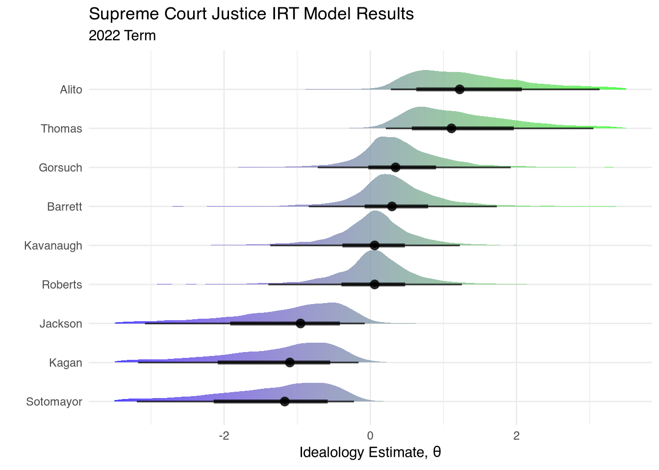
What should we take away from the ideology estimates from the model above? First, the ordering roughly matches intuition. We have the three liberal, Democrat-appointed, justices Sotomayor, Kagan, and Jackson receiving left-wing ideology scores. Kavanaugh and Roberts are considerably more right-wing than those three, followed by Barrett and Gorsuch. And Thomas and Alito are even more extreme in their conservatism compared to their other four Republican-appointed colleagues.

A second takeaway is that these estimates contain a lot of uncertainty. The theta posteriors for each justice are quite wide, especially for those on the ideological periphery. This is largely due to a lack of data. We are only examining a single year of Supreme Court cases (55 total in the model), and we only have nine individuals who are taking positions on these cases. IRT models produce more confident results as both items and responses increase. In principle we could extend this analysis back further in time by incorporating data on more Supreme Court terms. However, this is not necessarily a good idea because the ideological composition of the Court’s docket changes every year.

This leads us to the third takeaway. Be careful when extrapolating these results to the broader political context. An ideology score of 0 on this scale should not be construed as “centrist” or “moderate”! The Supreme Court docket is not a representative sample of the political issues facing the country each year. Justices on the Court choose to grant certiorari to only a small proportion of potential cases—a process which biases the ideological landscape of cases in a given term. If justice ideology impacts how they decide cases, it should also impact how they select which cases to decide in the first place. Furthermore, selection bias can occur at the lower court stage. Conservative activists are more likely to appeal extremist cases up to this incarnation of the Supreme Court because they know they have a better shot at winning on these issues compared to past terms. Conversely, liberal activists may not bother trying to get favorable cases on the court’s docket because they know they stand no chance.

So what do these results say about the 3-3-3 vs 6-3 debate?⁸ Perhaps it’s actually more of a 3-4-2 Court. That’s not to say that the four in the middle are true centrists though—they are simply slightly more moderate than Thomas and Alito (a very low bar).

4 Conclusion

To conclude, pack the court.

sessionInfo()

R version 4.4.0 (2024-04-24)
Platform: aarch64-apple-darwin20
Running under: macOS Sonoma 14.3

Matrix products: default
BLAS:   /Library/Frameworks/R.framework/Versions/4.4-arm64/Resources/lib/libRblas.0.dylib 
LAPACK: /Library/Frameworks/R.framework/Versions/4.4-arm64/Resources/lib/libRlapack.dylib;  LAPACK version 3.12.0

locale:
[1] en_US.UTF-8/en_US.UTF-8/en_US.UTF-8/C/en_US.UTF-8/en_US.UTF-8

time zone: America/Los_Angeles
tzcode source: internal

attached base packages:
[1] stats     graphics  grDevices utils     datasets  methods   base     

other attached packages:
[1] rstan_2.35.0.9000       StanHeaders_2.35.0.9000 ggdist_3.3.2           
[4] ggplot2_3.5.1           tidybayes_3.0.6         brms_2.21.6            
[7] Rcpp_1.0.12             dplyr_1.1.4            

loaded via a namespace (and not attached):
 [1] svUnit_1.0.6          tidyselect_1.2.1      farver_2.1.2         
 [4] loo_2.8.0.9000        fastmap_1.1.1         tensorA_0.36.2.1     
 [7] digest_0.6.36         lifecycle_1.0.4       processx_3.8.4       
[10] magrittr_2.0.3        posterior_1.6.0       compiler_4.4.0       
[13] rlang_1.1.4           tools_4.4.0           utf8_1.2.4           
[16] yaml_2.3.8            data.table_1.15.4     knitr_1.47           
[19] labeling_0.4.3        bridgesampling_1.1-2  htmlwidgets_1.6.4    
[22] bit_4.0.5             pkgbuild_1.4.4        curl_5.2.1           
[25] here_1.0.1            plyr_1.8.9            cmdstanr_0.8.0.9000  
[28] abind_1.4-5           withr_3.0.0           purrr_1.0.2          
[31] grid_4.4.0            stats4_4.4.0          fansi_1.0.6          
[34] colorspace_2.1-0      inline_0.3.19         scales_1.3.0         
[37] cli_3.6.3             mvtnorm_1.2-5         rmarkdown_2.26       
[40] crayon_1.5.2          generics_0.1.3        RcppParallel_5.1.8   
[43] rstudioapi_0.16.0     reshape2_1.4.4        tzdb_0.4.0           
[46] stringr_1.5.1         bayesplot_1.11.1.9000 parallel_4.4.0       
[49] matrixStats_1.3.0     vctrs_0.6.5           V8_4.4.2             
[52] Matrix_1.7-0          jsonlite_1.8.8        hms_1.1.3            
[55] arrayhelpers_1.1-0    bit64_4.0.5           tidyr_1.3.1          
[58] glue_1.7.0            codetools_0.2-20      ps_1.7.7             
[61] distributional_0.4.0  stringi_1.8.4         gtable_0.3.5         
[64] QuickJSR_1.3.0        munsell_0.5.1         tibble_3.2.1         
[67] pillar_1.9.0          htmltools_0.5.8.1     Brobdingnag_1.2-9    
[70] R6_2.5.1              rprojroot_2.0.4       vroom_1.6.5          
[73] evaluate_0.23         lattice_0.22-6        readr_2.1.5          
[76] backports_1.5.0       rstantools_2.4.0.9000 coda_0.19-4.1        
[79] gridExtra_2.3         nlme_3.1-164          checkmate_2.3.1      
[82] xfun_0.44             forcats_1.0.0         pkgconfig_2.0.3      

Footnotes

1. IRT can also be used on non-individual units, such as organizations, but most examples use individual people.

2. The no-ideological-difference-among-items assumption is pretty much always wrong, yet researchers continue to use additive index scales of latent variables in the social sciences all time. Do better! It’s not that hard!

3. Which is confusing because there are two parameters in the model: \(\theta\) and \(\xi\). Note that \(\theta\) in Equation 2 is not formulated exactly the same as the additive index \(\theta\) in Equation 1. In Equation 2 \(\theta\) is simply an arbitrary parameter for the latent variable as opposed to the scaled proportion of conservative votes as in Equation 1. We can, however, still interpret larger values of \(\theta\) as more conservative and lower values of \(\theta\) as more liberal.

4. A note on notation: in the dozens of books/articles I’ve read on IRT modeling, I have not found even two which share the same Greek letters for the ability, difficulty, and discrimination parameters. Sometimes \(\alpha\) is in place of \(\theta\). Sometimes \(\beta\) is in place of \(\xi\). The \(\gamma\) parameter can be any number of letters. I have decided to contribute to this ongoing mess and confusion by using my own “\(\gamma_j\theta_i + \xi_j\)”, whose exact permutation I have not seen anywhere else.

5. Long data is in contrast to “wide” data in a vote matrix—where the rows are justices and the columns are cases. Older IRT estimation packages, such as pscl, prefer data in the form a vote matrix.

6. See Bürkner 2020 for a comprehensive introduction in IRT modeling using brms.

7. CmdStanR is not the default backend for brms, but I prefer it to RStan because the output is more concise and it seems to sample faster.

8. Technically the 3-3-3 advocates are trying to put the nine justices on a two-dimensional scale, as opposed to the unidimensional left-right scale in our IRT model. They call their second fake second scale “institutionalism”. Technically we could add another dimension to our IRT model, but there is nothing in the data that explicitly codes cases as either pro-institutionalist or anti-institutionalist so there is not really a principled way of going about this.