Rats are “public enemy number one”—at least according to New York City Mayor Eric Adams. Last year the city established a “Rat Czar” who has been tasked with detecting and exterminating rat populations across the five boroughs. While I respect the lives all creatures great and small, mapping out the concentration of rats in the city seems like a worthwhile public service.

In this project I develop the NYC Rat Index using geospatial analysis in R. We will walk through some GIS wrangling steps and then employ Bayesian modeling to measure rat activity across New York. Use these results to figure out which neighborhoods to avoid—or which to seek out—depending on your overall disposition towards wild rodents.

# Packages used:
library(dplyr)
library(lubridate)
library(tidyr)
library(tidycensus)
library(purrr)
library(ggplot2)
library(MetBrewer)
library(spdep)
library(sf)
library(INLA)
library(leaflet)

Rat Data

Our data for constructing the Rat Index comes from the NYC Rat Information Portal (RIP).

rats <- readr::read_csv(here::here("posts", "nyc-rats", "data-raw", "Rodent_Inspection_20240528.csv")) |> 
  janitor::clean_names()

Each of the 2.5 million observations is a rodent inspection from the year 2010 to present. A lot of inspections don’t find evidence of rats, so we will focus only the rows where result == "Rat Activity". Mapping rat populations with this data is a bit problematic because rodent inspections are not random. The RIP discusses this in their disclaimer:

Notes on data limitations: Please note that if a property/taxlot does not appear in the file, that does not indicate an absence of rats - rather just that it has not been inspected. Similarly, neighborhoods with higher numbers properties with active rat signs may not actually have higher rat populations but simply have more inspections.

We can deal with some of this bias by building a geospatial model of rat activity—rather than by simply using the raw data on its own. The idea here is that we infer rat activity in areas with low inspection rates by how proximate they are to areas with high rat activity/inspection rates in the data. Given the fact that rats love scurrying around from place to place, let’s try to account for this spatial correlation statistically.

data_years <- 2015:2021

Although the rat data ranges from 2010 to present, we’ll restrict our analysis to between 2015 and 2021 because we’ll need to incorporate Census data later which is only available for this period.

rats_zip <- rats |> 
  mutate(year = year(mdy_hms(inspection_date)),
         # some ZIPs got put into the wrong boroughs
         borough = case_when(zip_code == 10463 ~ "Bronx",
                             zip_code == 10451 ~ "Bronx",
                             zip_code == 11370 ~ "Queens",
                             zip_code == 11207 ~ "Brooklyn",
                             .default = borough)) |> 
  summarise(n_rats = sum(result == "Rat Activity", na.rm = TRUE),
            .by = c("zip_code", "borough", "year")) |> 
  filter(year %in% data_years, !is.na(borough))

Let’s start by creating a new data frame, rats_zip, which collapses the number of rat activity observations (n_rats) down to the ZIP code-year level. We’ll use ZIP code as the level of spatial aggregation because most people know which ZIP code they live in (as opposed to Census tract or other designation). This will make it easier for New Yorkers to know the Rat Index value where they live. The downside of using ZIP codes, however, is that they are constructed to facilitate mail delivery—not balanced geospatial analysis.¹

get_rat_predictors <- function(year) {
  zip_data <- get_acs(
    geography = "zcta",
    variables = c("n_kitchens" = "B25051_002",
                  "n_food_workers" = "C24050_040",
                  "buildings_before_1939" = "B25034_011",
                  "total_population" = "B01003_001"),
    year = year,
    survey = "acs5",
    output = "wide",
    progress = FALSE
  )
  return(zip_data)
}

Next, let’s grab ZIP code covariates using the get_acs() function in the tidycensus R package. These are variables from the Census American Community Survey (ACS) which I believe can help predict rat activity in our model. Because most of my knowledge about rat psychology comes from the movie Ratatouille, the number of kitchens and the number of food workers (e.g. chefs) seem like they will be very important. The number of old buildings (built before 1939) in a ZIP code also seems relevant. I envision rats having an easier time infiltrating older buildings compared to new ones. And lastly we’ll use the total population variable because apparently rats like living near us humans.

nyc_rat_vars <- split(data_years, data_years) |> 
  map(get_rat_predictors) |> 
  list_rbind(names_to = "year") |> 
  mutate(zip_code = as.numeric(GEOID),
         year = as.numeric(year)) |> 
  filter(zip_code %in% rats_zip$zip_code)

Because our rat data is a time-series, we’ll run the partial function get_rat_predictors() over each year in data_years using purrr::map(). Ideally we would use the ACS 1-year file for each of these years, but ZIP code data is only available in the ACS 5-year file.

nyc_zips <- tigris::zctas(progress = FALSE) |> 
  mutate(zip_code = as.numeric(ZCTA5CE20)) |> 
  filter(zip_code %in% rats_zip$zip_code)

In addition to the outcome variable n_rats, and the Census covariates used to predict rat activity, we need the geospatial geometry of each ZIP code. Ideally we could get this information using the option geometry = TRUE in get_acs(). But I found that the ZIP code geometries had minuscule differences from year to year, which made any subsequent analysis with them a huge pain. So instead we will pull the spatial geometry data just once using the zctas() function in the tigris package.

# Merge the ZIP data in with the rats data
rats_all <- rats_zip |> 
  inner_join(nyc_rat_vars, by = c("zip_code", "year")) |> 
  left_join(nyc_zips, by = "zip_code") |> 
         # model functions like data to be indexed as 1, 2, 3, etc
  mutate(zip_code_code = as.integer(as.factor(zip_code)),
         year_code = as.integer(as.factor(year)))

Lastly we merge all three data sources (rats, rat predictors, ZIP code geometry) into a single data frame called rats_all.

Geospatial Wrangling

To infer rat activity from proximate ZIP codes, we need to know which ZIP codes are neighbors.

# Using only zip codes, boroughs, and geometry to illustrate the neighbor graph
zips_only <- rats_all |> 
  st_as_sf() |> 
  select(zip_code, borough) |> 
  distinct()

# Neighbor adjacency graph
zips_adj <- poly2nb(zips_only)

The function poly2nb() from the spdep package takes our data containing spatial geometry polygons and returns a neighbor adjacency graph. This tells us, for each ZIP code in our data, which ZIP codes touch it at at least one point. We could take a look at this network graph using the base plot(zips_adj) method, but I prefer the look and flexibility of ggplot.

nb_to_sf <- function(nb_obj, sf_obj) {
  sf_out <- as(nb2lines(nb_obj, coords = coordinates(as_Spatial(sf_obj))), "sf") |> 
    st_set_crs(st_crs(sf_obj))
  return(sf_out)
}

The function nb_to_sf() can be used to convert zips_adj back into an sf data object which plays nicely with ggplot functions.

ggplot(zips_only) +
  geom_sf(color = 'white', aes(fill = borough)) +
  geom_sf(data = nb_to_sf(zips_adj, zips_only)) +
  scale_fill_manual(values = met.brewer("Hokusai3")) + 
  theme_void()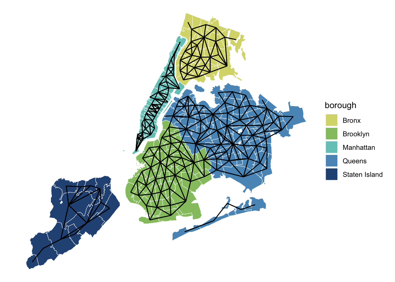

Here is our beautiful NYC ZIP code adjacency graph! Unfortunately for us, however, the poly2nb() function only connected ZIP codes if they were terrestrial neighbors. This leaves all the boroughs except Brooklyn and Queens disconnected from one another. The Rockaway beach area is also isolated from the rest of the city, and poor Roosevelt Island is all alone with zero neighbors. We need to do some adjustments if we want to properly model rat activity. While I’m not sure whether a rat could swim across the East River from Manhattan to Brooklyn, I have first hand knowledge of them traveling across the city’s various tunnels and bridges.

add_neighbors <- function(nb_obj, links, node_vec) {
  for (i in seq_along(links)) {
    nb_obj[[match(names(links[i]), node_vec)]] <- setdiff(as.integer(sort(c(nb_obj[[match(names(links[i]), node_vec)]], match(links[i], node_vec)))), 0)
    nb_obj[[match(links[i], node_vec)]] <- setdiff(as.integer(sort(c(nb_obj[[match(links[i], node_vec)]], match(names(links[i]), node_vec)))), 0)
  }
  return(nb_obj)
}

It turns out that adding manual connections to a nb spatial neighbors object is extremely annoying. The spdep package supposedly has a function for this: edit.nb(), but you will get an error saying “do not use in RStudio” (???). I refuse to work out of the Console like a caveman, so instead I wrote a function add_neighbors() to help with this. Enter your original nb spatial neighbors object, a vector of neighbor pairs you wish to connect, and the geography variable from the data frame you used to create the nb object—and you will get out a new nb spatial neighbors object with all those nodes connected. The links argument in this example will be ZIP code pairs and the node_vec argument will be the ZIP code column in zips_only, but add_neighbors() will also work if you want to connect Census tracts or any other geographic unit.

connect_nyc_neighbor_zips <- partial(
  add_neighbors,
  links = c("11414" = "11693", # Cross Bay Blvd
            "11234" = "11697", # Marine Parkway Bridge
            "10305" = "11209", # Verrazzano Bridge
            "10004" = "11231", # Brooklyn-Battery Tunnel
            "10038" = "11201", # Brooklyn Bridge
            "10002" = "11201", # Manhattan Bridge
            "10002" = "11211", # Williamsburg Bridge
            "10017" = "11109", # Queens-Midtown Tunnel
            "10022" = "11101", # Queensboro Bridge
            "10044" = "11106", # Roosevelt Island Bridge
            "10035" = "11102", # Triborough Bridge
            "10035" = "10454", # Triborough Bridge
            "10037" = "10451", # Madison Ave. Bridge
            "10039" = "10451", # 145th St. Bridge
            "10033" = "10453", # Washington Bridge
            "10034" = "10468", # University Heights Bridge
            "10034" = "10463", # Broadway Bridge
            "10465" = "11360", # Throgs Neck Bridge
            "10465" = "11357") # Whitestone Bridge
)

Because we will use add_neighbors() multiple times in this project, I created a purrr::partial() version of it with the major NYC bridges and tunnels connected by default. Now I know what you are thinking. What about the SUBWAY?! Rats LOVE the SUBWAY! Sorry, but it was tedious enough looking up all these bridges. A serious GIS specialist could probably do something fancy like overlay a shapefile of the NYC subway system on top of the ZIP code shapefile, and add connections that way. But for now we will just assume that rats are banned from riding the subway.

zips_adj_c <- zips_adj |> 
  connect_nyc_neighbor_zips(node_vec = zips_only$zip_code)

With that caveat out of the way let’s create a new spatial neighbor object, zips_adj_c, with the ZIP codes that we want connected.

ggplot(zips_only) +
  geom_sf(color = "white", aes(fill = borough)) +
  geom_sf(data = nb_to_sf(zips_adj_c, zips_only), color = "red") +
  geom_sf(data = nb_to_sf(zips_adj, zips_only)) +
  scale_fill_manual(values = met.brewer("Hokusai3")) + 
  theme_void()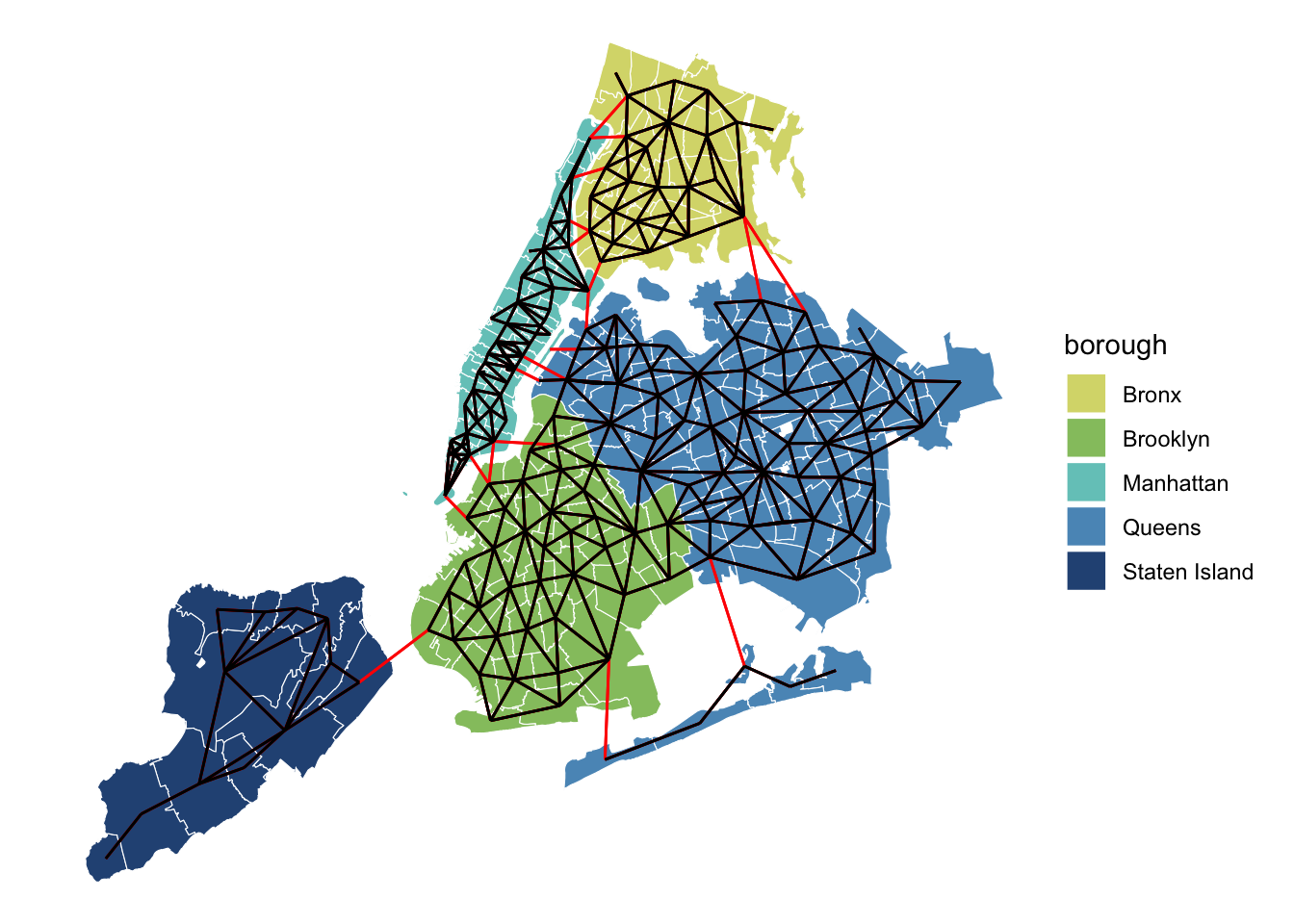

Plotting these two graphs on top of each other confirms that we fully connected the entire city! The rats will now be free to roam from borough to borough in our model.

Modeling the Rats

Let’s return to the ZIP-year level data, rats_all for constructing the Rat Index.

zips_adj_long <- rats_all |> 
  st_as_sf() |> 
  poly2nb() |> 
  connect_nyc_neighbor_zips(node_vec = rats_all$zip_code)

zip_mat <- nb2mat(zips_adj_long, style = "B")

We’ll create an nb spatial neighbor object from this long data using poly2nb() as before, and add the tunnel and bridge connections using connect_nyc_neighbor_zips(). We will then encode the neighbor relations in zips_adj_long as an adjacency matrix using nb2mat() with style = "B" for “binary”. This creates a square matrix of 1’s and 0’s where the 1’s denote adjacency between ZIP codes. The adjacency matrix is how we encode neighbor relations in the modeling step.

rat_mod = inla(
  n_rats ~ total_populationE + buildings_before_1939E + n_kitchensE + n_food_workersE +
    f(zip_code_code, model = "bym2", graph = zip_mat),
  data = rats_all,
  family = "poisson"
)

Time to build the rat model. We’ll use the INLA package to predict rat activity given the population, building age, kitchens, and food worker variables we assembled earlier. INLA is very popular for fitting Bayesian models with spatial components. It uses a form of approximate Bayesian inference called Itegrated Nested Laplace Approximation, which means it runs a lot faster than full Markov Chain Monte Carlo samplers such as Stan.

The f(zip_code_code, model = "bym", graph = zip_mat) section in the model is the spatial component. The part of the model that allows neighboring ZIP codes to share rat information with each other. INLA and all the spatial functions we used in spdep (poly2nb() and nb2mat()) are kind of old-school when it comes to their reliance on integer indexing—as opposed to allowing ZIP codes to be their true, un-ordered, selves. This is why I use the variable zip_code_code instead of zip_code here. It contains integer values matching each ZIP code with its position in the nb spatial neighbor object. The model = "bym2" part tells INLA we are doing spatial analyses using the Besag-York-Mollié method. BYM2 gives each ZIP code a varying intercept (i.e. “random effect”) which is a combination of spatial correlation with its neighboring ZIP codes and an unstructured effect for non-spatial rat behavior.

We’re using family = "poisson" in the model because the outcome variable, n_rats, is a count of rat inspections and Poisson likelihoods are good for count data.²

The Rat Index

rat_scores <- rats_all |> 
  mutate(rat_score = rat_mod$summary.fitted.values$mode) |> 
  st_as_sf() |> 
  summarise(rat_score = mean(rat_score),
            .by = c("zip_code", "borough"),
            across(geometry, st_union)) |> 
  mutate(log_rat_score = log10(rat_score),
         zip_rat_rank = as.integer(as.factor(-log_rat_score)),
         zip_rat_perc = percent_rank(-zip_rat_rank))

The predicted rat activity can be extracted from the fitted model using rat_mod$summary.fitted.values. Mean, median, and mode of these posterior values are all about the same, so we’ll save $mode as our new rat_score variable. Because rat_mod uses the time-series data, we will aggregate rat scores across years down to the ZIP code level. Rat activity is highly skewed, so for plotting purposes we’ll use log_rat_score. And we’ll also create rat index rank and percentile variables so that we can find the biggest rat hot-spots in the city.

l <- st_as_sf(rat_scores) |> 
  leaflet() |> 
  addTiles()

labels <- sprintf(
  "<strong> ZIP Code: %s </strong> <br/>
  Rat Index: %s <br/> Percentile: %s",
  rat_scores$zip_code, 
  round(rat_scores$rat_score, 2),
  round(rat_scores$zip_rat_perc, 3)
) |> 
  lapply(htmltools::HTML)

pal <- colorNumeric(
  palette = "plasma",
  domain = rat_scores$log_rat_score)

l |> 
  addPolygons(
    smoothFactor = .1, fillOpacity = .8,
    fillColor = ~pal(log_rat_score),
    weight = .1,
    highlightOptions = highlightOptions(weight = 5, color = "white"),
    label = labels,
    labelOptions = labelOptions(
      style = list(
        "font-weight" = "normal",
        padding = "3px 8px"
      ),
      textsize = "15px", direction = "auto"
    )
  ) |> 
  addLegend(
    pal = pal, values = ~log_rat_score, opacity = 1,
    labFormat = labelFormat(transform = function(x) 10^x),
    title = "Rat Index", position = "bottomright")

Here are the rats! Using the leaflet package we can put together a nice interactive map of rat activity across New York City. Mouse over any ZIP code and zoom in to see the raw rat index score and its rat percentile.

rat_scores |> 
  as_tibble() |> 
  arrange(zip_rat_rank) |> 
  select(borough, zip_code, rat_score, zip_rat_rank) |> 
  distinct() |> 
  head(n = 10)

# A tibble: 10 × 4
   borough   zip_code rat_score zip_rat_rank
   <chr>        <dbl>     <dbl>        <int>
 1 Brooklyn     11216     1320.            1
 2 Brooklyn     11237     1209.            2
 3 Brooklyn     11221     1167.            3
 4 Bronx        10457     1050.            4
 5 Brooklyn     11206      968.            5
 6 Bronx        10458      950.            6
 7 Bronx        10456      834.            7
 8 Bronx        10468      672.            8
 9 Bronx        10453      647.            9
10 Manhattan    10002      612.           10

Taking a look at the top 10 rat index ZIP codes, the major rat activity is in a handful of neighborhoods in parts of Brooklyn and the Bronx. Rats appear to be less prevalent as you move out to Staten Island or Queens in the peripheral areas of the city. But keep in mind that the data in this project leaves a lot to be desired. To quote a friend with whom I was discussing this project: “the rats are everywhere, even if the rat inspections haven’t been documented.”

sessionInfo()

R version 4.4.0 (2024-04-24)
Platform: aarch64-apple-darwin20
Running under: macOS Sonoma 14.3

Matrix products: default
BLAS:   /Library/Frameworks/R.framework/Versions/4.4-arm64/Resources/lib/libRblas.0.dylib 
LAPACK: /Library/Frameworks/R.framework/Versions/4.4-arm64/Resources/lib/libRlapack.dylib;  LAPACK version 3.12.0

locale:
[1] en_US.UTF-8/en_US.UTF-8/en_US.UTF-8/C/en_US.UTF-8/en_US.UTF-8

time zone: America/Los_Angeles
tzcode source: internal

attached base packages:
[1] stats     graphics  grDevices utils     datasets  methods   base     

other attached packages:
 [1] leaflet_2.2.2    INLA_24.05.01-1  sp_2.1-4         Matrix_1.7-0    
 [5] spdep_1.3-3      sf_1.0-16        spData_2.3.0     MetBrewer_0.2.0 
 [9] ggplot2_3.5.1    purrr_1.0.2      tidycensus_1.6.3 tidyr_1.3.1     
[13] lubridate_1.9.3  dplyr_1.1.4     

loaded via a namespace (and not attached):
 [1] gtable_0.3.5       xfun_0.43          htmlwidgets_1.6.4  tigris_2.1        
 [5] lattice_0.22-6     tzdb_0.4.0         crosstalk_1.2.1    vctrs_0.6.5       
 [9] tools_4.4.0        generics_0.1.3     curl_5.2.1         parallel_4.4.0    
[13] tibble_3.2.1       proxy_0.4-27       fansi_1.0.6        pkgconfig_2.0.3   
[17] KernSmooth_2.23-22 RColorBrewer_1.1-3 uuid_1.2-0         lifecycle_1.0.4   
[21] farver_2.1.1       fmesher_0.1.5      compiler_4.4.0     stringr_1.5.1     
[25] deldir_2.0-4       MatrixModels_0.5-3 munsell_0.5.1      janitor_2.2.0     
[29] snakecase_0.11.1   htmltools_0.5.8.1  class_7.3-22       yaml_2.3.8        
[33] jquerylib_0.1.4    pillar_1.9.0       crayon_1.5.2       classInt_0.4-10   
[37] wk_0.9.1           boot_1.3-30        tidyselect_1.2.1   rvest_1.0.4       
[41] digest_0.6.35      stringi_1.8.3      labeling_0.4.3     splines_4.4.0     
[45] rprojroot_2.0.4    fastmap_1.1.1      grid_4.4.0         here_1.0.1        
[49] colorspace_2.1-0   cli_3.6.2          magrittr_2.0.3     utf8_1.2.4        
[53] e1071_1.7-14       readr_2.1.5        withr_3.0.0        scales_1.3.0      
[57] rappdirs_0.3.3     bit64_4.0.5        timechange_0.3.0   rmarkdown_2.26    
[61] httr_1.4.7         bit_4.0.5          hms_1.1.3          evaluate_0.23     
[65] knitr_1.46         viridisLite_0.4.2  s2_1.1.6           rlang_1.1.3       
[69] Rcpp_1.0.12        glue_1.7.0         DBI_1.2.2          xml2_1.3.6        
[73] vroom_1.6.5        rstudioapi_0.16.0  jsonlite_1.8.8     R6_2.5.1          
[77] units_0.8-5

Footnotes

In Manhattan, 42 buildings have their own ZIP code.↩︎
No rats were poissoned during the fitting of this model.↩︎