# Loading in the packages used
library(tidyverse)
library(rvest)
library(MetBrewer)
library(ggdist)
library(brms)
library(distributional)
library(geomtextpath)
library(tidybayes)

# Global plotting theme for ggplot
theme_set(theme_ggdist())

# Set global rounding options
options(scipen = 1,
digits = 3)Does Height Matter When Running for President?
Height is supposed to confer all sorts of advantages in life. Taller people make more money, have an easier time finding romantic partners, and can reach things off the highest shelves without using a step stool. But does height matter when it comes to politics? The topic has been the subject of extensive debate—so much so that a Wikipedia page was written to provide information on the heights of US presidential candidates. In this post I analyze this debate quantitatively using R and Bayesian regression methods. My results conclusively show that height probably doesn’t matter much when it comes to winning the presidency.
Getting the data
The first thing to do is gather the data on presidential candidate heights. The package rvest is a great way to scrape the Wikipedia page above. It’s pretty easy to get data off Wikipedia because the HTML is relatively simple. But tables of data on Wikipedia need a bit of cleaning before they can be used for any statistical analysis. You have to remove things like citation markers, as well as fix column names and make sure columns containing numbers are actually numeric types.
url <- "https://en.wikipedia.org/wiki/Heights_of_presidents_and_presidential_candidates_of_the_United_States"

height_table <- url |>
  # Parse the raw html
  read_html() |>
  # Pull out the table elements
  html_elements("table") |>
  purrr::pluck(5) |>
  # Turn the candidate height table into a tibble
  html_table()

heights <- height_table |>
  # Assign names to all columns to fix duplicate originals
  `colnames<-`(c("election", "winner", "winner_height_in", "winner_height_cm",
               "opponent", "opponent_height_in", "opponent_height_cm",
               "difference_in", "difference_cm")) |>
  # Removing problematic elections
  filter(!election %in% c("1912", "1860", "1856", "1836", "1824"),
         opponent_height_cm != "") |>
  # Cleaning up the citation markers and fixing column types
  mutate(across(everything(),
                ~ str_remove_all(., "\\[.*\\]")),
         across(contains("_cm"),
                ~ str_remove_all(.x, "\\D") |>
                  as.numeric()),
         # Making a few new variable for the analysis
         winner_difference_cm = winner_height_cm - opponent_height_cm,
         winner_taller = if_else(winner_difference_cm > 0, 1, 0))
In the process of cleaning the presidential candidate height data I decided to remove all elections in which more than two candidates ran (1824, 1836, 1856, 1860, 1912), all elections in which a candidate’s height was missing from Wikipedia (1816: Rufus King, 1868: Horatio Seymour), and all uncontested elections (1788 and 1792: George Washington, 1820 James Monroe). No information regarding a height advantage can be gleaned from the latter two categories (unless it was Washington’s large stature that helped dissuade any potential challengers) so their exclusion should be uncontroversial. The removal of multi-candidate elections, however, was a choice I made in order to simplify the analysis. The role of height in a multi-candidate election is less straightforward than in a two-candidate election. Should we suppose voters simply gravitate towards the tallest candidate running? Or are they making height comparisons between all three candidates at once? Because political science lacks a good theory to support any of these explanations I dropped multi-candidate elections and moved on.
After these cleaning steps I made a new variable called winner_taller which simply denotes whether that taller candidate won the particular election, 1 or lost, 0. Using mean(heights$winner_taller) we see that the proportion of elections won by the taller candidate is 0.551. The taller candidate wins more on average! Skeptical readers will object that the sample size is too low for this result to be conclusive. “What is the standard error of the proportion!” they will say, “I want to see a p-value!” These are valid critiques, but as a fervent Bayesian I refuse to calculate any p-values. Let’s move on to some further analysis.
Presidential candidates compared to the general population
The original candidate height data set was at the election-level, meaning that every row represented a presidential election year. In order to look at candidate heights individually, I transformed the data into “long” format such that each row represents a single candidate. With the data at the candidate-level, we can now investigate how the heights of presidential candidates compare to the overall population.
heights_long <- heights |>
  pivot_longer(cols = c("winner", "opponent"),
               values_to = "candidate",
               names_to = "status") |>
  # Creating a single variable for candidate height
  mutate(height_cm = case_when(status == "winner" ~ winner_height_cm,
                               status == "opponent" ~ opponent_height_cm))
The graph below shows the distribution of candidate heights compared to the US adult male population. The variable “height” is often used to illustrate a Normal distribution in action. But technically, the Normal distribution does not accurately reflect height unless we first narrow the population down. Children and adults do not share the same height distribution, and neither do different genders. Each country, or region of the globe, likely also has a distinct height distribution. So unless we clearly define which population we’re talking about, “height” is best characterized as a mixture of normal distributions. Since almost all US presidential candidates have been adult men, however, I overlaid only the distribution for US adult males (mean 178 cm, standard deviation 8 cm).
heights_long |>
  select(height_cm, candidate) |>
  distinct() |>
  ggplot() +
  stat_function(geom = "textpath", vjust = 0, hjust = .2,
                label = "US Male Population",
                fun = function(x) dnorm(x, mean = 178, sd = 8) * 20) +
  geom_dots(aes(x = height_cm,
                fill = candidate == "Hillary Clinton",
                group = NA),
            size = .1) +
  scale_fill_manual(values = met.brewer("Lakota", 2)) +
  xlim(150, 200) +
  labs(x = "Height in cm", y = "",
       title = "Heights of US Presidential Candidates\nCompared to US Male Population") +
  theme(legend.position = "none",
        axis.line.y = element_blank(),
        axis.text.y = element_blank())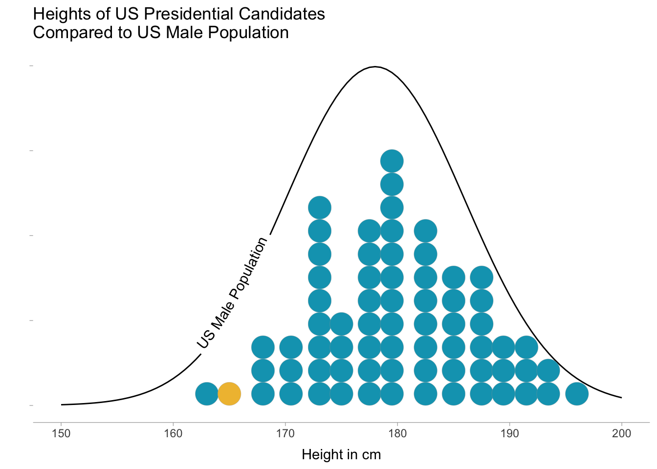
Hillary Clinton (represented by the yellow dot in the candidate distribution) should not be compared to the average US male in terms of height—but interestingly, isn’t the shortest candidate in US history. That honor goes to James Madison at 163 cm (5’ 4”). The graph shows that presidential candidates roughly align with overall male population heights. Perhaps candidates are slightly taller than the average US male, but the difference appears small.
How much does height contribute to winning the presidency?
Okay, so we discovered that the taller candidate wins slightly more often on average, but how does raw height affect a candidate’s chances of becoming president? To answer this question, we need to add a new dummy variable to our candidate-level data set indicating whether they won or lost.
heights_long <- heights_long |>
  mutate(winner = if_else(status == "winner", 1, 0))
Then I fit the following Bayesian logistic regression model to the data:
\[\begin{equation*} \begin{aligned} \text{Winner}_i &\sim \text{Bernoulli}(p) \\ p &= \text{logit}^{-1}(\alpha + \beta \ \text{Height}_i) \\ \alpha &\sim \text{Normal}(0, 2) \\ \beta &\sim \text{Normal}(0, 2) \end{aligned} \end{equation*}\]
There’s nothing too fancy going on in this model—just a standard logistic regression with a binary outcome (winning the presidency or not winning the presidency). The Normal(0, 2) priors on the intercept and slope coefficients are weakly informative, meaning they are wide enough to let the data inform our results, but narrow enough to be skeptical of extreme values. Given background knowledge of height in presidential campaigns, it’s unlikely it has a big effect on the outcome.
The code below fits the model using the brms package in R. Because the data only contain 96 candidate observations, the MCMC chains converge extremely quickly. Only 1.2 seconds for 12,000 iterations! Good practice when working with Bayesian models dictates that we look into the diagnostic measures (R-hat, effective sample size, number of divergent transitions, etc) of our fitted model. But since this model is very simple, I hope you will trust me that the fitting process worked reliably well.
height_model <- brm(
  winner ~ 1 + height_cm,
  prior = prior(normal(0, 2), class = "b") +
          prior(normal(0, 2), class = "Intercept"),
  family = bernoulli(link = "logit"),
  data = heights_long,
  seed = 111,
  refresh = 0,
  iter = 12000,
  backend = "cmdstanr"
)
Start samplingRunning MCMC with 4 sequential chains...
Chain 1 finished in 0.2 seconds.
Chain 2 finished in 0.2 seconds.
Chain 3 finished in 0.2 seconds.
Chain 4 finished in 0.2 seconds.
All 4 chains finished successfully.
Mean chain execution time: 0.2 seconds.
Total execution time: 1.3 seconds.Attempting to directly interpret coefficient values from logit models is rarely a good idea. Instead we can graph the results and compare the predicted probabilities of the outcome variable (winning the presidency) against a range of input variable values (candidate height in cm). This is what the (logit dotplot)[https://www.barelysignificant.com/post/glm/] below shows. The dots on the top and bottom of the graph represent candidates that either won or lost, and the line between them shows what our model predicts the winning probability to be at each height value on the x-axis. the weakly upward slope on this prediction line tells us that there is barely any benefit to being an extra cm taller when it comes to winning a presidential election.
# Generate a set of values across the range of the height data
prediction_grid <- with(heights_long,
  data.frame(height_cm = seq(min(height_cm), max(height_cm), length.out = 100))
)

prediction_grid |>
  # Generate posterior draws
  add_epred_draws(height_model, ndraws = 100) |>
  # Collapse down to the height level
  group_by(height_cm) |>
  summarise(.median = median(.epred),
            .sd = sd(.epred)) |>
  # Convert log odds into predicted probabilities
  mutate(log_odds = dist_normal(.median, .sd),
         p_winner = dist_transformed(log_odds, plogis, qlogis)) |>
  ggplot(aes(x = height_cm)) +
  geom_dots(
    aes(y = winner, side = ifelse(winner == 1, "bottom", "top")),
    scale = 0.4,
    fill = "#931e18",
    size = .1,
    data = heights_long) +
  stat_lineribbon(
    aes(ydist = p_winner), alpha = .25, fill = "#931e18", size = .5) +
  labs(title = "Predicted Probability of Winning the Presidency\nBased on Candidate Height",
       x = "Height cm",
       y = "Pr(Winning)")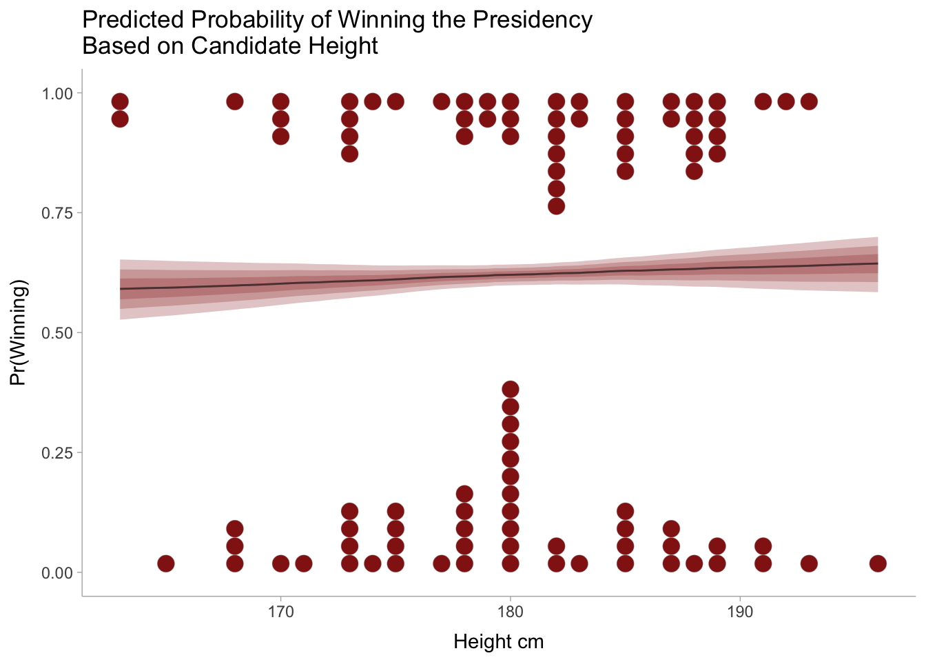
Apparently height has little effect on the probability that a candidate wins the presidency. But what if the candidate was extremely tall? It is now time to make a confession. The true reason I started this project was for selfish reasons. As someone who is 206 cm tall (6’ 9”), I wanted to know what my chances were of becoming president based only on my height. Plugging my 206 cm into the logistic regression model produces the posterior probability distribution shown in the graph below. While there is considerable uncertainty due to the small sample size of candidates, the model says I have between a 60 and 70% chance to win. Amazing!
prediction_grid <- with(heights_long,
  data.frame(height_cm = 206)
)

prediction_grid |>
  add_epred_draws(height_model, ndraws = 12000) |>
  mutate(p_winner = 1 / (1 + exp(-.epred))) |>
  ggplot(aes(x = p_winner)) +
  stat_slabinterval(fill = "#04a3bd", trim = FALSE) +
  labs(title = "Posterior Probability of Winning\nfor Someone Very Tall",
       x = "Pr(Winning | Height = 206 cm)",
       y = "") +
  theme(axis.line.y = element_blank(),
        axis.text.y = element_blank())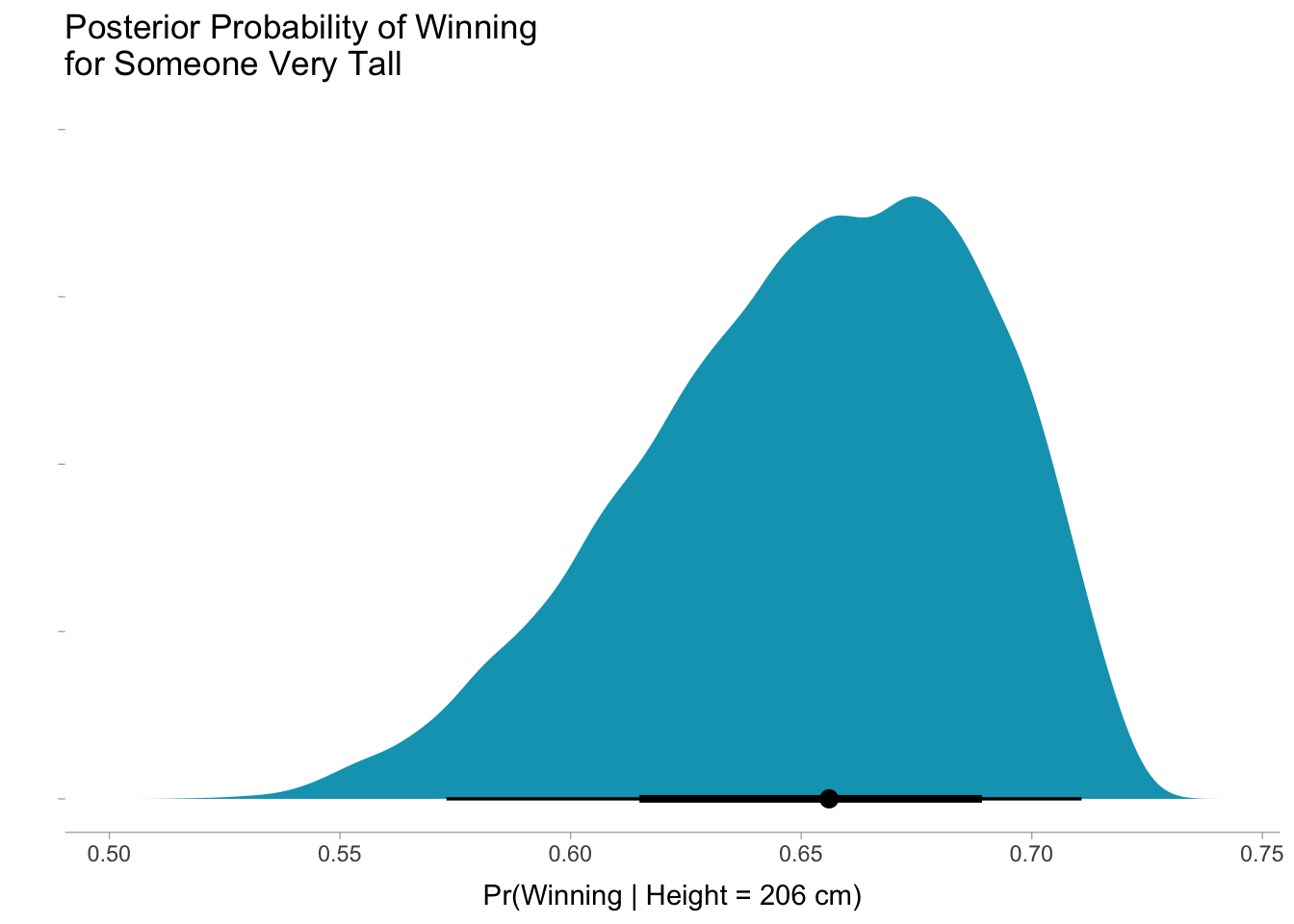
As we all know, numbers don’t lie. So keep an eye out for the Bert–2024 campaign coming soon.
Session info
sessionInfo()R version 4.1.1 (2021-08-10)
Platform: x86_64-apple-darwin17.0 (64-bit)
Running under: macOS Big Sur 10.16
Matrix products: default
BLAS: /Library/Frameworks/R.framework/Versions/4.1/Resources/lib/libRblas.0.dylib
LAPACK: /Library/Frameworks/R.framework/Versions/4.1/Resources/lib/libRlapack.dylib
locale:
[1] en_US.UTF-8/en_US.UTF-8/en_US.UTF-8/C/en_US.UTF-8/en_US.UTF-8
attached base packages:
[1] stats graphics grDevices utils datasets methods base
other attached packages:
[1] tidybayes_3.0.2.9000 geomtextpath_0.1.0 distributional_0.3.0
[4] brms_2.17.4 Rcpp_1.0.8.3 ggdist_3.0.99.9000
[7] MetBrewer_0.2.0 rvest_1.0.2 forcats_0.5.1
[10] stringr_1.4.0 dplyr_1.0.9 purrr_0.3.4
[13] readr_2.1.2 tidyr_1.2.0 tibble_3.1.7
[16] ggplot2_3.3.6 tidyverse_1.3.1
loaded via a namespace (and not attached):
[1] readxl_1.3.1 backports_1.4.1 systemfonts_1.0.3
[4] selectr_0.4-2 plyr_1.8.7 igraph_1.3.1
[7] svUnit_1.0.6 splines_4.1.1 crosstalk_1.2.0
[10] rstantools_2.2.0 inline_0.3.19 digest_0.6.29
[13] htmltools_0.5.2 fansi_1.0.3 magrittr_2.0.3
[16] checkmate_2.1.0 tzdb_0.2.0 modelr_0.1.8
[19] RcppParallel_5.1.5 matrixStats_0.62.0 xts_0.12.1
[22] prettyunits_1.1.1 colorspace_2.0-3 textshaping_0.3.6
[25] haven_2.4.3 xfun_0.31 callr_3.7.0
[28] crayon_1.5.1 jsonlite_1.8.0 lme4_1.1-27.1
[31] zoo_1.8-10 glue_1.6.2 gtable_0.3.0
[34] emmeans_1.7.2 V8_4.2.0 pkgbuild_1.3.1
[37] rstan_2.26.11 abind_1.4-5 scales_1.2.0
[40] mvtnorm_1.1-3 DBI_1.1.1 miniUI_0.1.1.1
[43] viridisLite_0.4.0 xtable_1.8-4 stats4_4.1.1
[46] StanHeaders_2.26.11 DT_0.23 htmlwidgets_1.5.4
[49] httr_1.4.2 threejs_0.3.3 arrayhelpers_1.1-0
[52] posterior_1.2.1 ellipsis_0.3.2 pkgconfig_2.0.3
[55] loo_2.5.1 farver_2.1.0 dbplyr_2.1.1
[58] utf8_1.2.2 labeling_0.4.2 tidyselect_1.1.2
[61] rlang_1.0.2 reshape2_1.4.4 later_1.3.0
[64] munsell_0.5.0 cellranger_1.1.0 tools_4.1.1
[67] cli_3.3.0 generics_0.1.2 broom_0.8.0
[70] ggridges_0.5.3 evaluate_0.15 fastmap_1.1.0
[73] yaml_2.3.5 processx_3.5.3 knitr_1.39
[76] fs_1.5.2 nlme_3.1-152 mime_0.12
[79] projpred_2.0.2 xml2_1.3.2 compiler_4.1.1
[82] bayesplot_1.9.0 shinythemes_1.2.0 rstudioapi_0.13
[85] curl_4.3.2 gamm4_0.2-6 reprex_2.0.1
[88] stringi_1.7.6 ps_1.7.0 Brobdingnag_1.2-7
[91] lattice_0.20-44 Matrix_1.3-4 nloptr_1.2.2.2
[94] markdown_1.1 shinyjs_2.1.0 tensorA_0.36.2
[97] vctrs_0.4.1 pillar_1.7.0 lifecycle_1.0.1
[100] bridgesampling_1.1-2 estimability_1.3 data.table_1.14.2
[103] httpuv_1.6.5 R6_2.5.1 promises_1.2.0.1
[106] gridExtra_2.3 codetools_0.2-18 boot_1.3-28
[109] colourpicker_1.1.1 MASS_7.3-54 gtools_3.9.2.1
[112] assertthat_0.2.1 withr_2.5.0 shinystan_2.6.0
[115] mgcv_1.8-36 parallel_4.1.1 hms_1.1.1
[118] grid_4.1.1 coda_0.19-4 minqa_1.2.4
[121] cmdstanr_0.4.0 rmarkdown_2.14 shiny_1.7.1
[124] lubridate_1.7.10 base64enc_0.1-3 dygraphs_1.1.1.6